If you've been tuned into space weather for any amount of time, then you've probably seen geomagnetic storm forecasts from the NOAA Space Weather Prediction Center (SWPC) posted on social media hyping up certain events and aurora possibilities.
After seeing these posts, you may ask yourself, "What are those?" or "How accurate are those forecasts?" and maybe even "How do they make those predictions?" Well, the short answer is that these geomagnetic storm predictions are created from CME model outputs, but the majority of the time, the models, how they work, and most importantly, their uncertainties, are not communicated in the forecast that ends up blasted all over social media.
In this blog, I'll walk you through how coronal mass ejections (CMEs) are modeled and worked into geomagnetic storm forecasts and introduce you to the HUXt model - a user-friendly platform for monitoring space weather events from the Sun to the Earth.
What are CMEs?
Coronal mass ejections are explosions of plasma from the Sun out into space. These plasma clouds are like sun sneezes, but instead of mucus (gross), CMEs are full of charged particles (like electrons and protons) and carry with them a magnetic field, usually in the form of a (flux) rope or slinky. While other space weather phenomena like coronal holes can give us relatively-predictable geomagnetic storms, CMEs occur suddenly. They can occur without warning and take 1-3 days to travel to Earth if directed our way.

Many CMEs occur in connection with solar flares - solar flares are bursts of light from active regions and sunspot groups. They can release large chunks of the Sun’s atmosphere as CMEs. Solar flares and CMEs are two phenomena that are related, but not the same. Some solar flares occur without launching CMEs, and some CMEs occur from random locations on the Sun or from prominences/filaments without accompanying solar flares or over active regions. Typically, X-class solar flares (the strongest level) will be accompanied by CMEs, but not all the time!

CMEs can also create geomagnetic storms of all sizes. Weak ejections may be barely detectable at Earth, but dense and fast plasma clouds can create strong events when they impact our magnetic shield (magnetosphere).

Tracking CMEs
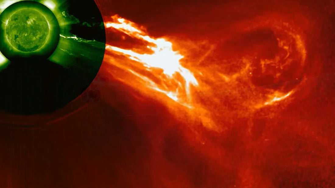
Tracking a CME in space is difficult. Typically, when one of these plasma clouds leaves the Sun’s surface, it quickly accelerates and expands. By examining images of the Sun taken in ultraviolet wavelengths, scientists can study the Sun’s upper atmosphere called the corona. This is the same layer we see when the moon blocks the Sun during a total solar eclipse. In fact, one of the earliest observations of a CME occurred during a solar eclipse when a large loop of light was seen slowly moving out from the Sun. A telltale sign a CME has occurred on the Sun is a “dimming” in the corona. This occurs when plasma has been evacuated from the Sun’s atmosphere, leaving a sort of burn scar behind. Sometimes, these dimmings look just like that, dimmings. Other times, you can actually see a shock wave propagating through the Sun’s atmosphere like waves rippling through water. They are beautiful to watch!

When a CME leaves the Sun’s inner corona and heads out into space, we switch to an instrument called a “coronagraph” to measure the speed and direction of the plasma cloud. While a total solar eclipse allows us to see the Sun’s outer atmosphere, they only happen about once per year and only for a few minutes. Luckily, in space, we have permanent solar eclipses in the form of coronagraphs. Currently, the only coronagraph instruments are LASCO onboard the SOHO spacecraft and COR2 onboard STEREO-A. Soon, the CCOR coronagraph instrument onboard GOES-19 will come online.

A coronagraph measures the scattered light (a phenomenon called Thomson scattering) from solar wind flowing away from the Sun. When a dense cloud emerges (like a CME), they appear as whitish blobs. The speeds of these CMEs in coronagraph imagery are measured by automatic routines and manually by space weather forecasters as inputs to models. How bright these clouds appear tell forecasters about the density of these ejections. The direction of these CMEs coming off the Sun determine where they may be directed within the solar system. Since the satellites containing the coronagraph instruments are located near Earth, any CMEs directly aimed at Earth will appear as clouds expanding like a halo around the solar disk. Halos can be symmetric, asymmetric, full, or partial. A “halo CME” is one that forms the classic halo signature in coronagraph imagery. These halo CMEs then contain at least some Earth-directed part to them. So, they are what we look forward to potentially causing geomagnetic storms if and when they impact our planet’s magnetosphere.

CME models
While some aurora chasers may prefer to do their own analysis of solar imagery to determine the arrival times and directionalities of CMEs, sophisticated models in combination with analysis from professional space weather forecasters offer the most accurate estimates of where CMEs will go when they leave the Sun. For aurora chasing purposes, we are most interested in if a CME will hit Earth and when it will arrive.
CME models take in information from solar imagery, like the source location of the explosion in the Sun’s atmosphere and the speed, brightness, and angular width of the plasma cloud as seen in coronagraphs. CMEs and these initial parameters can be detected using automated tools (e.g., CACTus), or in the case of most space weather offices, on-call forecasters monitoring the Sun use computer tools to measure these ejections. Once these values are plugged into models, because a CME is a plasma, it won’t simply travel in a straight line like a bullet leaving the Sun. Complicated equations take into account interactions of the plasma cloud with the Sun’s atmosphere as it expands and accelerates into the solar wind.

There are many CME models that exist, and some of them are operational meaning they are used by space weather forecasters to process events in (near) real-time. For example, the WSA-ENLIL model is used by the NASA M2M and NOAA SWPC offices, 3DCORE is used by the Austrian Space Weather Office, and EUHFORIA is used by the European Space Agency. The HUXt model is another model, and because of some specific features, it’s my favorite, especially when trying to understand uncertainties in forecasts. Let’s explore HUXt, explain what it is and how to use it, and hopefully make this tool an integral part of your aurora chasing efforts.
What is HUXt?
HUXt (Heliospheric Upwind eXtrapolation with time dependence) is a solar wind model developed by one of the Heliophysics teams from University of Reading. It can be used to predict CMEs from the Sun - their arrival times and speeds as well as to show the uncertainty of these predictions.
View the latest HUXt prediction here.

HUXt uses the same CME data, such as speed, source location on the solar surface, and equations as several other CME models. But what HUXt does differently is perform these calculations several hundred times to include different conditions the CME can encounter on its way to Earth. These conditions include slower or faster ambient solar wind through which the CME travels. A good analogy is trying to drive across town with or without traffic. HUXt takes into account many different “traffic” scenarios for CMEs coming off the Sun headed towards Earth that may cause the plasma cloud to arrive earlier or later. This technique is called ensemble modeling. The result is a forecast dashboard that looks like this:

How to use HUXt
The HUXt forecast dashboard has five main fields. Here is the breakdown of all of them.
① Time series of solar wind speed

What is it?
This plot is the main part of the forecast. Part of the plot in the white area is the predicted solar wind speed with several lines and different shading for probabilities. Gray is the time prior to the forecast, with prior prediction as well as solar wind speed registered by the DSCOVR satellite (shown in red). Real-time DSCOVR data can be a bit unreliable, so it is primarily used for HUXt forecast verification.
The black line on the plot is the predicted CME speed by the Met Office Space Weather Operations Centre. The black dashed line is the solar wind speed without any influence from a CME. The tan line is the median for all the results when different conditions are used for modeling. Shaded areas represent the spread of results for different conditions. They are given in percentiles and coded by different colors. Narrow color bands mean high confidence in the forecast. Wide bands represent low confidence in the forecast.
How do I use this data?
CME arrival time is notoriously difficult to predict with good accuracy. The HUXt forecast can be used to estimate the interval when a CME can be expected to arrive at Earth as well as the speed at the time of arrival. A CME with a faster speed means less travel time as well as a more significant impact. It also translates into a greater probability of aurora shortly after the CME arrives and starts to interact with Earth’s magnetic shield (magnetosphere).
② CME arrival probability at Earth

What is it?
This plot covers the probability of CME arrival(s) at Earth within a certain time window. Each CME is coded by a different color. A broad and low peak to one of these curves means low probability of arrival and low confidence in the arrival time. A narrow and tall peak means high probability of arrival and high confidence in arrival time.
How do I use this data?
This plot helps answer two burning questions about CME forecasting: “When will the CME come?” and “How sure are we that it is coming?” Tall narrow peaks indicate high chances that something is coming. Be ready to watch the solar wind data when the time of arrival is approaching.
③ Table of the Earth-directed CME properties and forecast arrival times/speeds

What is it?
This is a table of all CMEs with a possible Earth-directed component in the HUXt forecast with corresponding color codes and the following CME characteristics: time, speed, location on the map of solar wind, and width. The table lists the percent of modeled results where the CME was forecasted as arriving at Earth (hit %) as well as the estimated arrival time and margin of error (+/-).
How do I use this data?
Look for CMEs with a high probability of arrival. These are a lot more likely to have an impact than low-probability CMEs that may completely miss Earth. Check the predicted time of arrival as well as the interval to start planning for a potential geomagnetic storm. Of course, we never know if a CME has hit us until we detect its signature in satellites at L1, but it is still good to be prepared for action.
④ Summary of the input data

What is it?
This is a map of solar wind some distance away from, and looking at, the Sun. The map is generated at a distance of 21.5 solar radii, to be exact. This is where the solar wind is assumed to go ``supersonic” and is thus a good input for model boundary conditions This is like taking a roadtrip in your car and using your cruising highway speed to calculate how long it will take for you to arrive at your destination. You wouldn’t use the speed as you accelerate on the onramp since you haven’t reached the cruising speed you will be at for most of your trip. It just so happens that the “onramp” for solar wind is about 21.5 solar radii long. The CME ``footprint” is given by the color assigned to that CME in the table seen in ③. CMEs that are no longer in the forecast appear as gray circles. Earth is the dot in the center of the map that may or may not be within the CME circle.
How do I use this data?
Look for CMEs that have Earth within their “footprint”. They are more likely to produce an impact and a resulting geomagnetic disturbance leading to aurora. CMEs with the “footprint” grazing Earth may pass close enough for the magnetosphere to feel the shock and minor impact.
⑤ The probability density of CME arrival speeds, for the Earth-impacting CMEs only

What is it?
This is a plot of confidence in predicted CME speeds at the time of arrival. Higher confidence levels will be reflected as narrower peaks.
How do I use this data?
Faster CMEs are more likely to have a stronger impact. Look for CMEs with higher speeds and narrow peaks as prime candidates to produce stronger geomagnetic disturbances which can in turn lead to stronger auroral displays.
Just as any other current model, HUXt can not perfectly predict CMEs. Solar wind leaving the Sun has a long way to travel before it arrives at Earth, and current observational or tracking tools do not generate sufficient data for accurate modeling. Any forecast remains a possibility until the CME is detected by one of the space weather satellites at L1 (at Earth). The ground-truth data of aurora also come from live sightings and sky cameras, not from solar wind data at L1 Once a CME hits upstream monitors, it still needs to interact with Earth’s magnetosphere which can funnel energy from the solar wind into the aurora through complicated mechanisms outside the scope of a CME model.
Why is HUXt important for aurora chasing?
CME models are used by space weather forecasting offices to issue geomagnetic storm watches. For example, NOAA SWPC, the official forecasting agency for the United States, will use the WSA-ENLIL model and simulate conditions at Earth like the density, speed, and magnetic field strength for a CME when it arrives. A faster and denser CME, or a train of CMEs may trigger more severe geomagnetic storm watches. For example, during the May 10-13, 2024 Gannon Storm, a train of relatively strong CMEs were modeled by WSA-ENLIL prompting NOAA SWPC to issue a G4 (Kp 8) geomagnetic storm watch.

What’s important to understand about these models and the resulting geomagnetic storm watches is that they all have inherent uncertainty. Particularly, this uncertainty lies in their CME arrival time predictions. HUXt lets you see more of the inner workings of the model and better communicates these error bars. Most models have arrival time uncertainties around +/- 7 hours, but sometimes, if the confidence of a direct CME hit is low or it is predicted to combine or interact with other solar wind structures (e.g., CMEs or high speed streams), this +/- uncertainty may be 12+ hours.

While you can find my full space weather event “workflow” in my Beginner’s Guide to Aurora Chasing e-book, generally, when I see a CME has occurred on the Sun, I will go through the following motions:
- Check solar imagery (i.e., EUV and coronagraph) of the event to see if it “passes the eye test.” Sometimes it’s nice to actually observe the CME on the Sun and in the coronagraph imagery to add context to the models. I will also check whether the CME was a full or partial halo and if any direction has more ejecta. In other words, is the CME Earth-directed, and is all of it heading at us, or just some of it? Since I have been looking at CMEs for quite some time and have even written papers on CME modeling, I have a trained eye for analyzing these images, but if you find it too difficult, just skip this step and move to the next.
- Check the HUXt forecast. Make a note of the impact time and the uncertainty. It’s important to also convert the impact time from UTC to your local time zone. I use a time converter app to help me. If the CME impact has a low velocity (300-600 km/s), it likely won’t cause as much of a disturbance as one with a high velocity (600+ km/s). How strong the CME is predicted to be and the arrival time uncertainty and model confidence % will determine how excited I get about an event.
- Check what other people are saying. HUXt is just one model. NASA and NOAA release their own models along with other groups. It’s helpful to not only get the spread of arrival times for one model, but the “spread of spreads” across many models. The NASA Coordinated Community Modeling Center (CCMC) has a CME Scoreboard where different space weather offices and research groups can upload their models of CMEs in real-time. You can then see how well different groups agree with each other. Arrival time uncertainties and model confidence percentages are also given by some of these other models.
- Check the NOAA SWPC forecast discussions and 3-day geomagnetic outlook and Kp forecast. This tells me how strong the CME(s) may be when it reaches Earth (according to the NOAA SWPC modeling efforts, at least). Of course, Kp is not an indicator of potential auroral strength, but I will get more excited about a Kp 8 watch than a Kp 5 watch, for example. If you don’t know the limitations of Kp, read my beginner’s guide e-book or check out my aurora forecasting blog post.
- Check other data sources like solar wind parameters at L1 (e.g., ACE EPAM low energy particles) to detect the shock passage of the CME. I start doing this on the early end of the +/- error bar in arrival time. When the CME arrives, then I kick into aurora monitoring mode and get ready to go out chasing! If the CME does not arrive after the end of the arrival time window, including uncertainty, then I will conclude a “miss” and not prepare for any passage of that particular CME.

With all this information, I hope HUXt becomes a part of your aurora chasing workflow and you understand a bit more about how CMEs are modeled and their uncertainties. It’s important to realize the difficulty of generating accurate space weather forecasts and how to interpret CME models. The more you understand about what’s “under the hood” of geomagnetic activity forecasts and solar storm predictions, the more prepared you will be for aurora action when CMEs arrive at Earth.
This blog post was written by Vincent E. Ledvina with the HUXt tutorial mostly written by Dr. Tanya E. Melnik, Christian L. Harris, Margaret Sonnemann and Dr. Mathew J. Owens.